AlphaGo is quite famous when I was a freshman of college. It somehow is the reason that I was addicted to Reinforcement Learning. Thus Our journey of model-based RL will start here. Although it is not the first one that propose model-based RL, I still believe it will give a big picture of model-based RL.
Mastering the game of Go with deep neural networks and tree search
Introduction
AlphaGo combines 2 kinds of model, including policy network and value network. The policy network takes the board position as input and output the probability of next action of each position. The value network also take the board position as input and output the winner of the game.
We pass in the board position as a 19×19 image and use convolutional layers to construct a representation of the position. We use these neural networks to reduce the effective depth and breadth of the search tree: evaluating positions using a value network, and sampling actions using a policy network.
We train the model in 2 stage. In the first stage, we use supervised learning with KGS dataset to train the policy network to predict the next action of humans. Then, in the second stage, we use reinforment learning and self-play to train the model by themself.
Stage1: Supervised Learning of Policy Network
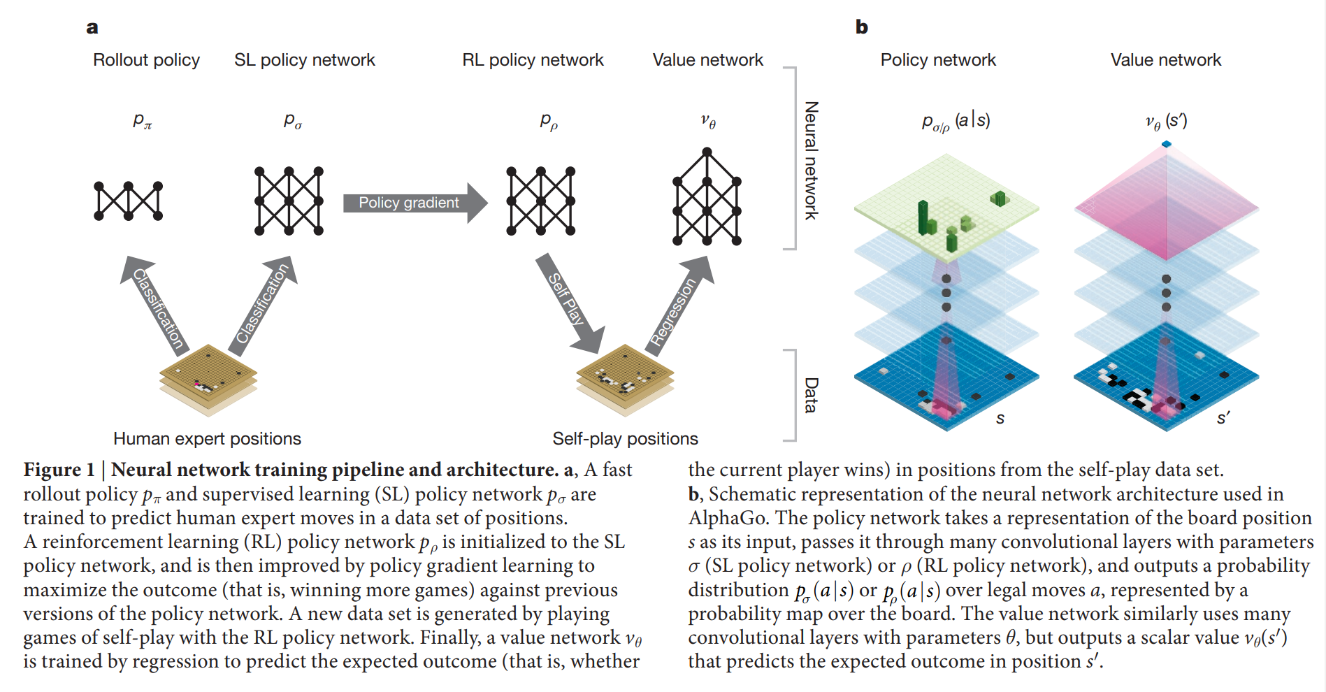
A fast rollout policy $p_{\pi}$ and supervised learning (SL) policy network $p_{\sigma}$ are trained to predict human expert moves in a data set of positions. The fast rollout policy $p_{\pi}$ is trained only with some important features such as Stone colour to reduce the complexity of the model(faster but less accurate) while the SL policy network $p_{\sigma}$ is trained with whole position of Go.
We trained a 13-layer policy network, which we call the SL policy network, from 30 million positions from the KGS Go Server. Then we update the policy network with the following function to maximize the probability of predicting the action of human experts:
$$ \triangle \sigma \propto \frac{\partial log \ p_{\sigma}(a|s)}{\partial \sigma} $$
Stage2: Reinforcement learning of policy networks
We use policy gradient reinforcement learning (RL) to update the network. The RL policy network $p_{\rho}$ is identical in structure to the SL policy network, its weights $\rho$ are initialized to the same values, $\rho = \sigma$. We play games between the current policy network $p_{\rho}$ and a randomly selected previous iteration of the policy network to prevent overfit and stablize training. To update the RL policy network, we use policy gradient to maximize the expected outcome:
$$ \triangle \rho \propto \frac{\partial log \ p_{\rho}(a_t|s_t)}{\partial \rho} z_t $$
Here we use a reward function $r(s)$ that t is 0 for all non-terminal time steps $t<T$. The outcome $z_t = \pm r(s_T)$ is the terminal reward at the end of the game if the current player wins, $r(s_T) = +1$, loses $r(s_T) = -1$.
Stage2: Reinforcement learning of value networks
Estimating a value function $v^p(s)$ that predicts the outcome from position $s$ of games played by using policy $p$ for both players
$$ v^p(s) = E[z_t | s_t = s, a_{t … T} \sim p] $$
We approximate the value function using a value network $v_{\theta}(s)$ with weights $\theta$, $v_{\theta}(s) \approx v^{p_{\rho}}(s) \approx v^*(s)$.
We define the loss function of the value network with mean squared error(MSE):
$$ \triangle \theta \propto \frac{\partial v_{\theta}(s)}{\partial \theta} (z - v_{\theta}(s)) $$
But how do we search the optimal value through policy network? There are 5 steps as Figure3:
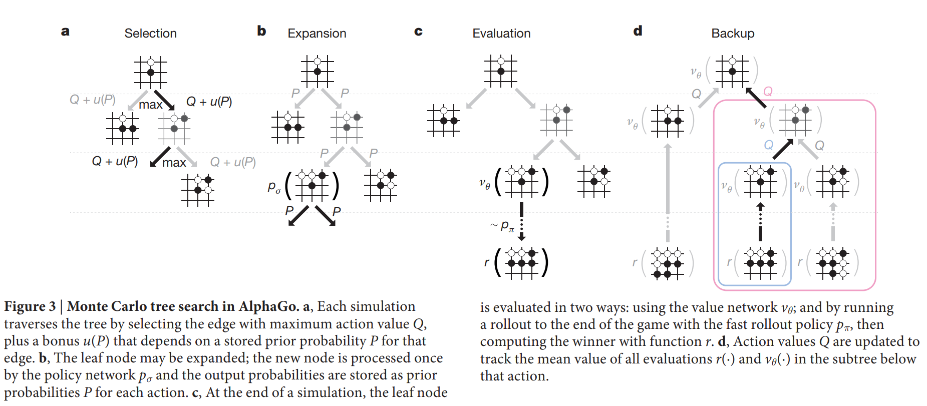
Step 1: Selection
Each simulation traverses the tree by selecting the edge with maximum action value $Q$, plus a bonus $u(P)$ that depends on a stored prior probability $P(s, a)$ for that edge.
Step 2: Expansion
The leaf node may be expanded. The new node is processed once by the policy network $p_{\sigma}$ with output $P(s, a)=p_{\sigma}(a|s)$.
Each edge $(s, a)$ of the search tree stores an action value $Q(s, a)$, visit count $N(s, a)$, and prior probability $P(s, a)$.
The $u(s, a)$ is a kind of bonus that is proportional to the prior probability but decays with repeated visits to encourage exploration.
At each time step $t$ of each simulation, an action $a_t$ is selected from state $s_t$
$$ a_t = \mathop{\arg\max}_a (Q(s_t, a) + u(s_t, a)) $$
so as to maximize action value plus a bonus
$$ u(s, a) \propto \frac{P(s, a)}{1 + N(s, a)} $$
Step 3: Evaluation
The leaf node is evaluated in two very different ways: first, by the value network $v_{\theta}(s_L)$; and second, by the outcome $z_L$ of a random rollout played out until terminal step $T$ using the fast rollout policy $p_{\pi}$; these evaluations are combined, using a mixing parameter $\lambda$, into a leaf evaluation $V(s_L)$.
$$ V(s_L) = (1 - \lambda) v_{\theta}(s_L) + \lambda z_L $$
Step 4: Backup
At the end of simulation, the action values and visit counts of all traversed edges are updated. Each edge accumulates the visit count and mean evaluation of all simulations passing through that edge as following:
$$ N(s, a) = \sum_{i = 1}^{n} 1(s, a, i) $$
$$ Q(s, a) = \frac{1}{N(s, a)} \sum_{i = 1}^{n} 1(s, a, i) V(s_L^i) $$
where $s_L^i$ is the leaf node from the ith simulation and $1(s, a, i)$ indicates whether an edge $(s, a)$ was traversed during the ith simulation.