A Review of SVM and SMO

Note: full code is on my github.

1. Abstract

In this article, I will derive SMO algorithm and the Fourier kernel approximation which are well-known algorithm for kernel machine. SMO can solve optimization problem of SVM efficiently and the Fourier kernel approximation is a kind of kernel approximation that can speed up the computation of the kernel matrix. In the last section, I will conduct a evaluation of my manual SVM on the simulation dataset and “Women’s Clothing E-Commerce Review Dataset”.

2. Sequential Minimal Optimization(SMO)

The SMO(Sequential Minimal Optimization) algorithm is proposed from the paper Sequential Minimal Optimization: A Fast Algorithm for Training Support Vector Machines in 1998 by J. Platt. In short, SMO picks 2 variables $\alpha_i, \alpha_j$ for every iteration, regulate them to satisfy KKT condition and, update them. In the following article, I will derive the whole algorithm and provide the evaluation on the simulation and real dataset.

We’ve known he dual problem of soft-SVM is

$$ \sup_{\alpha} \sum_{i=1}^{N} \alpha_i - \frac{1}{2} \sum_{i=1}^{N} \sum_{j=1}^{N} \alpha_i \alpha_j y_i y_j k(x_i, x_j) \ \newline \text{subject to} \ 0 \leq \alpha_i \leq C, \sum_{i=1}^{N} \alpha_i y_i= 0 $$

We also define the kernel.

$$ k(x_i, x_j) = \langle \phi(x_i), \phi(x_j) \rangle $$

where $\phi$ is an embedding function projecting the data points to a high dimensional space.

However, it’s very hard to solve because we need to optimize $N$ variables. As a result, J. Platt proposed SMO to solve this problem efficiently.

2.1 Notation

We denote the target function as $\mathcal{L}(\alpha, C)$

$$ \mathcal{L} (\alpha) = \sum_{i=1}^{N} \alpha_i - \frac{1}{2} \sum_{i=1}^{N} \sum_{j=1}^{N} \alpha_i \alpha_j y_i y_j k(x_i, x_j) $$

We also denote the kernel of $x_1, x_2$ as $K_{1, 2} = k(x_1, x_2)$.

2.2 Step 1. Update 2 Variable

First, we need to pick 2 variables to update in sequence, so we split the variables $\alpha_1, \alpha_2$ from the summation.

$$ \mathcal{L}(\alpha) = \alpha_1 + \alpha_2 - \frac{1}{2} \alpha_1^2 y_1^2 K_{1,1} - \frac{1}{2} \alpha_2^2 y_2^2 K_{2,2} \newline -\frac{1}{2} \alpha_1 \alpha_2 y_1 y_2 K_{1, 2} - \frac{1}{2} \alpha_2 \alpha_1 y_2 y_1 K_{2, 1} \newline -\frac{1}{2} \alpha_1 y_1 \sum_{i=3}^{N} \alpha_i y_i K_{i,1} -\frac{1}{2} \alpha_1 y_1 \sum_{i=3}^{N} \alpha_i y_i K_{1, i} \newline -\frac{1}{2} \alpha_2 y_2 \sum_{i=3}^{N} \alpha_i y_i K_{i,2} -\frac{1}{2} \alpha_2 y_2 \sum_{i=3}^{N} \alpha_i y_i K_{2, i} \newline +\sum_{i=3}^{N} \alpha_i - \frac{1}{2} \sum_{i=3}^{N} \sum_{j=3}^{N} \alpha_i \alpha_j y_i y_j k(x_i, x_j) $$

$$ = \alpha_1 + \alpha_2 - \frac{1}{2} \alpha_1^2 y_1^2 K_{1,1} - \frac{1}{2} \alpha_2^2 y_2^2 K_{2,2} - \alpha_1 \alpha_2 y_1 y_2 K_{1, 2} \newline -\alpha_1 y_1 \sum_{i=3}^{N} \alpha_i y_i K_{i,1} - \alpha_2 y_2 \sum_{i=3}^{N} \alpha_i y_i K_{i,2} + \mathcal{Const} $$

$$ = \alpha_1 + \alpha_2 - \frac{1}{2} \alpha_1^2 K_{1,1} - \frac{1}{2} \alpha_2^2 K_{2,2} - \alpha_1 \alpha_2 y_1 y_2 K_{1, 2} \newline -\alpha_1 y_1 \sum_{i=3}^{N} \alpha_i y_i K_{i,1} - \alpha_2 y_2 \sum_{i=3}^{N} \alpha_i y_i K_{i,2} + \mathcal{Const} $$

where $\mathcal{Const} = \sum_{i=3}^{N} \alpha_i - \frac{1}{2} \sum_{i=3}^{N} \sum_{j=3}^{N} \alpha_i \alpha_j y_i y_j k(x_i, x_j)$. We see it as a constant because it is regardless to $\alpha_1, \alpha_2$.

2.2.1 The Relation Between The Update Values and The Hyperplane

We’ve derive the partial derivative of the dual problem.

$$ \frac{\partial L(w, b, \xi, \alpha, \mu)}{\partial w} = w - \sum_{i=1}^N \alpha_i y_i x_i = 0 $$

We can get

$$ w = \sum_{i=1}^N \alpha_i y_i x_i $$

Thus, we can rewrite the hyperplane $f_{\phi}(x)$ with kernel.

$$ f_{\phi}(x) = w^{\top} \phi(x) + b = b + \sum_{i=1}^N \alpha_i y_i k(x_i, x) $$

The corresponding code:

1
2
def __f(self, i):
    return snp.dot((self.alpha * self.y), self.K[i, :]) + self.b

We also denote $v_1, v_2$ as

$$ v_1 = \sum_{i=3}^{N} \alpha_i y_i K_{i,1} = \sum_{i=1}^{N} \alpha_i y_i k(x_i, x_1) - \alpha_1^{old} y_1 k(x_1, x_1) - \alpha_2^{old} y_2 k(x_2, x_1) $$

$$ = f_{\phi}(x_1) - b - \alpha_1^{old} y_1 K_{1, 1} - \alpha_2^{old} y_2 K_{2, 1} $$

and $v_2$ is similar.

$$ v_2 = \sum_{i=3}^{N} \alpha_i y_i K_{i,2} = \sum_{i=1}^{N} \alpha_i y_i k(x_i, x_2) - \alpha_1^{old} y_1 k(x_1, x_2) - \alpha_2^{old} y_2 k(x_2, x_2) $$

$$ = f_{\phi}(x_2) - b - \alpha_1^{old} y_1 K_{1, 2} - \alpha_2^{old} y_2 K_{2, 2} $$

where $\alpha_1^{old}$ and $\alpha_2^{old}$ are $\alpha_1$ and $\alpha_2$ of the previous iteration. Since we see $\alpha_i, i \geq 3$ as constant, $\alpha_i$ shouldn’t depends on update variables $\alpha_1, \alpha_2$.

2.2.2 Rewrite The Complementary Slackness

The constraint can be represented as

$$ \sum_{i=1}^{N} \alpha_i y_i = \alpha_1 y_1 + \alpha_2 y_2 + \sum_{i=3}^{N} \alpha_i y_i = 0 $$

$$ \alpha_1 y_1 + \alpha_2 y_2 = - \sum_{i=3}^{N} \alpha_i y_i = \zeta $$

$$ \alpha_1 = \frac{\zeta - \alpha_2 y_2}{y_1} $$

Since $y_1$ is either 1 or -1, thus

$$ \alpha_1 = \zeta y_1 - \alpha_2 y_1 y_2 $$

The old ones are the same.

$$ \alpha_1^{old} = \zeta y_1 - \alpha_2^{old} y_1 y_2 $$

Replace the symbol $\alpha_1, v_1, v_2$

$$ \mathcal{L}(\alpha) = (\zeta y_1 - \alpha_2 y_1 y_2) + \alpha_2 \newline -\frac{1}{2} (\zeta y_1 - \alpha_2 y_1 y_2)^2 K_{1,1} - \frac{1}{2} \alpha_2^2 K_{2,2} - (\zeta y_1 - \alpha_2 y_1 y_2) \alpha_2 y_1 y_2 K_{1, 2} \newline -(\zeta y_1 - \alpha_2 y_1 y_2) y_1 v_1 - \alpha_2 y_2 v_2 $$

$$ = (\zeta y_1 - \alpha_2 y_1 y_2) + \alpha_2 \newline -\frac{1}{2} (\zeta^2 + \alpha_2^2 - 2 \zeta \alpha_2 y_2) K_{1,1} - \frac{1}{2} \alpha_2^2 K_{2,2} - (\zeta \alpha_2 y_2 - \alpha_2^2) K_{1, 2} \newline -(\zeta - \alpha_2 y_2) v_1 - \alpha_2 y_2 v_2 $$

2.2.3 Combine the $v_1$, $v_2$ and $\zeta$

$$ v_1 - v_2 = [ \ f_{\phi}(x_1) - b - \alpha_1^{old} y_1 K_{1, 1} - \alpha_2^{old} y_2 K_{2, 1} \ ] - [ \ f_{\phi}(x_2) - b - \alpha_1^{old} y_1 K_{1, 2} - \alpha_2^{old} y_2 K_{2, 2} \ ] $$

$$ = [ \ f_{\phi}(x_1) - b - ( \zeta y_1 - \alpha_2^{old} y_1 y_2) y_1 K_{1, 1} - \alpha_2^{old} y_2 K_{2, 1} \ ] - [ \ f_{\phi}(x_2) - b - ( \zeta y_1 - \alpha_2^{old} y_1 y_2) y_1 K_{1, 2} - \alpha_2^{old} y_2 K_{2, 2} \ ] $$

$$ = [ \ f_{\phi}(x_1) - f_{\phi}(x_2) \ ] + [ \ - ( \zeta - \alpha_2^{old} y_2) K_{1, 1} - \alpha_2^{old} y_2 K_{2, 1} \ ] - [ \ - ( \zeta - \alpha_2^{old} y_2) K_{1, 2} - \alpha_2^{old} y_2 K_{2, 2} \ ] $$

$$ = [ \ f_{\phi}(x_1) - f_{\phi}(x_2) \ ] + [ \ - \zeta K_{1, 1} + \alpha_2^{old} y_2 K_{1, 1} - \alpha_2^{old} y_2 K_{2, 1} \ ] - [ \ - \zeta K_{1, 2} + \alpha_2^{old} y_2 K_{1, 2} - \alpha_2^{old} y_2 K_{2, 2} \ ] $$

$$ = f_{\phi}(x_1) - f_{\phi}(x_2) - \zeta K_{1, 1} + \zeta K_{1, 2} + ( K_{1, 1} + K_{2, 2} - 2 K_{1, 2} ) \alpha_2^{old} y_2 $$

2.2.4 Derive Gradient of $\alpha_2$

$$ \frac{\partial \mathcal{L}(\alpha)}{\partial \alpha_2} = -y_1 y_2 + 1 - \frac{1}{2} (2 \alpha_2 - 2 \zeta y_2) K_{1,1} - \alpha_2 K_{2, 2} - (\zeta y_2 - 2 \alpha_2) K_{1, 2} - (- y_2) v_1 - y_2 v_2 $$

$$ = (- \alpha_2 K_{1, 1} - \alpha_2 K_{2, 2} + 2 \alpha_2 K_{1, 2}) + \zeta y_2 K_{1, 1}- \zeta y_2 K_{1, 2} - y_1 y_2 + y_2 v_1 - y_2 v_2 + 1 $$

$$ = -\alpha_2 (K_{1, 1} + K_{2, 2} - 2 K_{1, 2}) + \zeta y_2 K_{1, 1}- \zeta y_2 K_{1, 2} - y_1 y_2 + y_2(v_1 - v_2) + 1 $$

Replace $v_1 - v_2$ containing old $\alpha_1^{old}, \alpha_2^{old}$ (derived in 2.2.3)

$$ \frac{\partial \mathcal{L}(\alpha)}{\partial \alpha_2} = -\alpha_2 (K_{1, 1} + K_{2, 2} - 2 K_{1, 2}) + \zeta y_2 K_{1, 1}- \zeta y_2 K_{1, 2} - y_1 y_2 + y_2 [ \ f_{\phi}(x_1) - f_{\phi}(x_2) - \zeta K_{1, 1} + \zeta K_{1, 2} + ( K_{1, 1} + K_{2, 2} - 2 K_{1, 2}) \alpha_2^{old} y_2 \ ] + 1 $$

$$ = -(K_{1, 1} + K_{2, 2} - 2 K_{1, 2}) \alpha_2 + ( K_{1, 1} + K_{2, 2} - 2 K_{1, 2} ) \alpha_2^{old} + y_2 (f_{\phi}(x_1) - f_{\phi}(x_2) + y_2 - y_1) $$

Let $\eta$ and $E_i$ be

$$ \eta = K_{1, 1} + K_{2, 2} - 2 K_{1, 2}, \quad E_i = f_{\phi}(x_i) - y_i $$

$$ \frac{\partial \mathcal{L}_d(\alpha)}{\partial \alpha_2} = - \eta \alpha_2 + \eta \alpha_2^{old} + y_2 (E_1 - E_2) $$

Since we want to minimize the gradient, let the gradient be 0.

$$ -\eta \alpha_2 + \eta \alpha_2^{old} + y_2 (E_1 - E_2) = 0 $$

Then we can find the relation between new and old $\alpha_2$ as following

$$ \alpha_2 = \alpha_2^{old} + \frac{y_2 (E_1 - E_2)}{\eta} $$

To make the notation more clear to identify, we denote $\alpha_2^{new}$ as the new value of the update.

$$ \alpha_2^{new} = \alpha_2^{old} + \frac{y_2 (E_1 - E_2)}{\eta} $$

The corresponding code:

 1
 2
 3
 4
 5
 6
 7
 8
 9
10
11
def __E(self, i):
    return self.__f(i) - self.y[i]

def __eta(self, i, j):
    return self.K[i, i] + self.K[j, j] - 2 * self.K[i, j]

def __alpha_j_new(self, i, j):
    E_i = self.__E(i)
    E_j = self.__E(j)
    eta = self.__eta(i, j)
    return self.alpha[j] + (self.y[j] * (E_i - E_j) / eta), E_i, E_j, eta

2.3 Step 2. Clip with Bosk Constraint

The new values should satisfy the complementary slackness as

$$ \alpha_1 y_1 + \alpha_2 y_2 = \zeta, \quad 0 \leq \alpha_i \leq C $$

Since $y_1, y_2$ may have different labels, thus we consider 2 cases. The first case is $y_1 \neq y_2$ as the left part of the figure 1 and another case is $y_1 = y_2$ which corresponds to he right part of the figure.

Note that there is another line in quadrant 3 in the case 2 but it doesn’t show in the figure due to the limit of the size.

bosk constraint

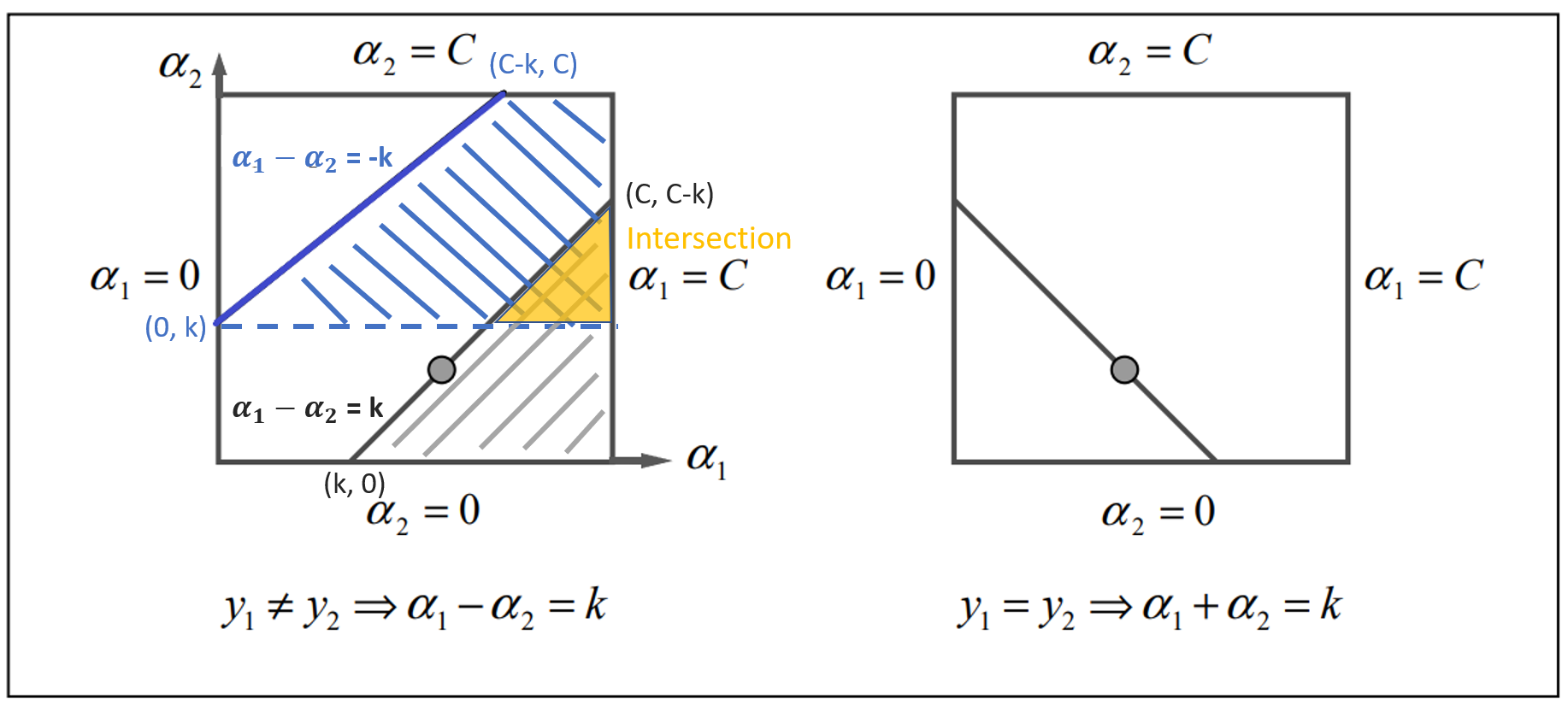
Figure 1

2.3.1 Case 1: Inequality

When $y_1 \neq y_2$, the equation is either $\alpha_1 - \alpha_2 = k$ or $\alpha_1 - \alpha_2 = -k$ where $k = |\zeta|$ is a positive constant.

First, we consider the blue area $\alpha_1 - \alpha_2 = -k$. We can see $\alpha_1 \in [C, k] = [C, \alpha_2 - \alpha_1]$. The upper bound should be $C$ and the lower bound should be $\alpha_2 - \alpha_1$.

$$ B_U = C, \ B_L = \alpha_2 - \alpha_1 $$

Next, we consider the grey area $\alpha_1 - \alpha_2 = k$. We can see $\alpha_1 \in [0, C-k] = [0, C + \alpha_2 - \alpha_1]$. The upper bound should be $C + \alpha_2 - \alpha_1$ and the lower bound should be 0.

$$ B_U = C + \alpha_2 - \alpha_1, \ B_L = 0 $$

Combine 2 cases, both new and old values should satisfy the bosk constraint. The upper bound of $\alpha_2^{new}$ can be written as

$$ B_U = \min(C, C + \alpha_2^{old} - \alpha_1^{old}) $$

and the lower bound is

$$ B_L = \max(0, \alpha_2^{old} - \alpha_1^{old}) $$

2.3.2 Case 2: Equality

When $y_1 = y_2$, the equation is either $\alpha_1 + \alpha_2 = k$ or $\alpha_1 + \alpha_2 = -k$ where $k$ is a positive constant.

In similar way, we can derive the case of equality. The upper bound can be written as

$$ B_U = \min(C, \alpha_2^{old} + \alpha_1^{old}) $$

and the lower bound is

$$ B_L = \max(0, \alpha_2^{old} + \alpha_1^{old} - C) $$

2.3.3 Clip The Value

According the bound we’ve derived, we need clip the updated variable $\alpha_2^{new}$ to satisfy the constraint. In addition, we denote the new value after clipping as $\alpha_2^*$.

$$ \alpha_2^* = CLIP(\alpha_2^{new}, B_L, B_U) $$

The corresponding code:

 1
 2
 3
 4
 5
 6
 7
 8
 9
10
11
12
def __bound(self, i, j):
        if self.y[i] == self.y[j]:
            B_U = min(self.C, self.alpha[j] + self.alpha[i])
            B_L = max(0, self.alpha[j] + self.alpha[i] - self.C)
        else:
            B_U = min(self.C, self.C + self.alpha[j] - self.alpha[i])
            B_L = max(0, self.alpha[j] - self.alpha[i])
        return B_U, B_L
def __update_alpha_j(self, i, j):
        B_U, B_L = self.__bound(i, j)
        alpha_j_star, E_i, E_j, eta = self.__alpha_j_new(i, j)
        return np.clip(alpha_j_star, B_L, B_U), E_i, E_j, eta

2.3.4 Update $\alpha_1$

We’ve know the complementary slackness.

$$ \alpha_1^* y_1 + \alpha_2^* y_2 = \alpha_1^{old} y_1 + \alpha_2^{old} y_2 = \zeta $$

Move the updated value $\alpha_1^*$ to the left side and we can get

$$ \alpha_1^* = \frac{\alpha_1^{old} y_1 + \alpha_2^{old} y_2 - \alpha_2^* y_2}{y_1} $$

$$ \alpha_1^* = \alpha_1^{old} + y_1 y_2(\alpha_2^{old} - \alpha_2^*) $$

The corresponding code:

1
2
def __update_alpha_i(self, i, j, alpha_j_star):
    return self.alpha[i] + self.y[i] * self.y[j] * (self.alpha[j] - alpha_j_star)

2.4 Step 3. Update Bias

The only equation that contains bias $b$ is the function $f_{\phi}(x) = b + \sum_{i=1}^N \alpha_i y_i k(x_i, x)$. When $0 \lt \alpha_i^* \lt C$, it means that the data point $x_i$ is right on the margin such that $f_{\phi}(x)=y_i$, $f_{\phi}^(x_i) = y_i$ and the bias $b_1^, b_2^$ can be derived directly. Note that for convenience, $f_{\phi}^(x_w) = \sum_{i=3}^N \alpha_i y_i K_{i, w} - \alpha_1^* y_1 K_{1, w} - \alpha_2^* y_2 K_{2, w} + b^* = y_w$ contains updated variables $\alpha_2^, \alpha_2^, b^*$.

If $0 < \alpha_1^* < C$, the data point $x_1$ should right on the margin and $f_{\phi}^*(x_1) = y_1$. The bias derived from $\alpha_1$.

$$ b_1^* = y_1 - \sum_{i=3}^N \alpha_i y_i K_{i, 1} - \alpha_1^* y_1 K_{1, 1} - \alpha_2^* y_2 K_{2, 1} $$

$$ = (y_1 - f_{\phi}(x_1) + \alpha_1^{old} y_1 K_{1, 1} + \alpha_2^{old} y_2 K_{2, 1} + b) - \alpha_1^* y_1 K_{1, 1} - \alpha_2^* y_2 K_{2, 1} $$

$$ = -E_1 - y_1 K_{1, 1} (\alpha_1^* - \alpha_1^{old}) - y_2 K_{2, 1} (\alpha_2^* - \alpha_2^{old}) + b $$

If $0 < \alpha_2^* < C$, the data point $x_2$ should right on the margin and $f_{\phi}^*(x_2) = y_2$. The bias derived from $\alpha_2$.

$$ b_2^* = y_2 - \sum_{i=3}^N \alpha_i y_i K_{i, 2} - \alpha_1^* y_1 K_{1, 2} - \alpha_2^* y_2 K_{2, 2} $$

$$ = (y_2 - f_{\phi}(x_2) + \alpha_1^{old} y_1 K_{1, 2} + \alpha_2^{old} y_2 K_{2, 2} + b) - \alpha_1^* y_1 K_{1, 2} - \alpha_2^* y_2 K_{2, 2} $$

$$ = -E_2 - y_1 K_{1, 2} (\alpha_1^* - \alpha_1^{old}) - y_2 K_{2, 2} (\alpha_2^* - \alpha_2^{old}) + b $$

When the data point $x_i, x_j$ are both not on the margin, we choose the average of $b_1^* \ and \ b_2^*$ as the updated value.

$$ b^* = \frac{b_1^* + b_2^*}{2} $$

The code of updating bias.

 1
 2
 3
 4
 5
 6
 7
 8
 9
10
11
12
13
def __update_b(self, i, j, alpha_i_star, alpha_j_star, E_i, E_j):
        b_star = 0
        b_i_star = -E_i - self.y[i] * self.K[i, i] * (alpha_i_star - self.alpha[i]) - self.y[j] * self.K[j, i] * (alpha_j_star - self.alpha[j]) + self.b
        b_j_star = -E_j - self.y[i] * self.K[i, j] * (alpha_i_star - self.alpha[i]) - self.y[j] * self.K[j, j] * (alpha_j_star - self.alpha[j]) + self.b

        if alpha_i_star <= self.C and alpha_i_star >= 0:
            b_star = b_i_star
        elif alpha_j_star <= self.C and alpha_j_star >= 0:
            b_star = b_j_star
        else:
            b_star = (b_i_star + b_j_star) / 2
        
        return b_star

For more detail, please see the pseudo code.

2.5 Pseudo Code

Given $C$, otherwise the default value is $C = 5$

Given $\epsilon$, otherwise the default value is $\epsilon = 10^{-6}$

Given $\text{max-iter}$, otherwise the default value is $\text{max-iter} = 10^{3}$

For all $\alpha_i = 0, 1 \leq i \leq N$

$b = 0$

$move = \infty$

while($move > \epsilon$ and $iter \leq \text{max-iter}$):

$\alpha_1^* = \alpha_2^* = b^* = move = 0$
for($n$ in $N/2$):
- Choose the index $i, j$ from 1 to $N$
- $E_i = f(x_i) - y_i$
- $E_j = f(x_j) - y_j$
- $\eta = K_{i, i} + K_{j, j} - 2 K_{i, j}$
- $\alpha_j^{new} = \alpha_j + \frac{y_j (E_i - E_j)}{\eta}$
  Bosk Constraint
- if($y_i = y_j$):
  - $B_U = \min(C, \alpha_j + \alpha_i)$
  - $B_L = \max(0, \alpha_j + \alpha_i - C)$
- else:
  - $B_U = \min(C, C + \alpha_j - \alpha_i)$
  - $B_L = \max(0, \alpha_j - \alpha_i)$
- $\alpha_j^* = CLIP(\alpha_j^{new}, B_L, B_U)$
- $\alpha_i^* = \alpha_i + y_i y_j(\alpha_j - \alpha_j^*)$
  Update Bias
- $b_i^* = - E_i - y_i K_{i, i} (\alpha_i^* - \alpha_i) - y_j K_{j, i} (\alpha_j^* - \alpha_j) + b$
- $b_j^* = - E_j - y_i K_{i, j} (\alpha_i^* - \alpha_i) - y_j K_{j, j} (\alpha_j^* - \alpha_j) + b$
- if($0 \leq \alpha_i \leq C$):
  - $b^* = b_i^*$
- else if($0 \leq \alpha_j \leq C$):
  - $b^* = b_j^*$
- else:
  - $b^* = \frac{b_i^* + b_j^*}{2}$
- $move = move + |\alpha_1^* - \alpha_1| + |\alpha_2^* - \alpha_2| + |b^* - b|$
- Let $\alpha_i = \alpha_i^* \quad \alpha_j = \alpha_j^* \quad b = b^*$
$iter = iter + 1$

Here is the Python code:

 1
 2
 3
 4
 5
 6
 7
 8
 9
10
11
12
13
14
15
16
17
18
19
20
21
22
23
24
25
26
27
28
29
30
31
32
33
34
35
36
37
38
39
40
41
42
43
44
45
46
47
48
49
50
51
def fit(self, X, y):
        self.X = np.array(X)
        self.y = np.reshape(np.array(y), (-1, ))
        self.n, self.dim = self.X.shape
        
        self.K = self.cal_kernel(self.X)

        self.alpha = np.zeros(self.n)
        self.b = 0

        iter = 0
        loss = np.inf
        move = np.inf

        while iter < self.max_iter and move > self.epsilon:
            loss = move = 0

            for i in range(self.n):
                j = self.__choose_j(i)

                alpha_j_star, E_i, E_j, eta = self.__update_alpha_j(i, j)
                if eta <= 0:
                    self.warning('Eta <= 0')
                    continue

                alpha_i_star = self.__update_alpha_i(i, j, alpha_j_star)
                if abs(alpha_j_star - self.alpha[j]) < 0.00001:
                    self.warning('alpha_j not moving enough')
                    continue

                b_star = self.__update_b(i, j, alpha_i_star, alpha_j_star, E_i, E_j)

                # Calculate the movement of alpha and b
                move = move + abs(alpha_i_star - self.alpha[i]) + abs(alpha_j_star - self.alpha[j]) + abs(b_star - self.b)

                # Update variables
                self.alpha[i] = alpha_i_star
                self.alpha[j] = alpha_j_star
                self.b = b_star
            
            # Calculate the loss
            loss = sum(map(lambda x: abs(self.__E(x)), np.arange(self.n)))
            # Calculate the accuracy
            acc = self.acc()
            self.loss_history.append(loss)
            self.move_history.append(move)
            self.acc_history.append(acc)

            # if not skip:
            iter += 1
            self.info("Iter: ", iter, " | Loss: ", loss, " | Move: ", move, " | Acc: ", acc)

3. Fourier Kernel Approximation

The Fourier kernel approximation is proposed from the paper Random Features for Large-Scale Kernel Machines on NIPS'07. It’s a widely-used approximation to accelerate the kernel computing especially for the high dimensional dataset. For a dataset with dimension $D$ and data points $N$, the time complexity of computing the exact kernel is $\mathcal{O}(DN^2)$ and the Fourier kernel approximation is $\mathcal{O}(SN^3)$ with $S$ samples. While the dimension goes up, the approximation remains the same computing time because it is regardless to the dimension of the dataset.

3.1 Bochner’s Theorem

If $\phi: \mathbb{R}^n \to \mathbb{C}$ is a positive definite, continuous, and satisfies $\phi(0)=1$, then there is some Borel probability measure $\mu \in \mathbb{R}^n$ such that $\phi = \hat{\mu}$

Thus, we can extend the Bochner’s theorem to kernel.

3.2 Theorem 1

According to Bochner’s theorem, a continuous kernel $k(x, y) = k(x-y) \in \mathbb{R}^d$ is positive definite if and only if $k(\delta)$ is the Fourier transform of a non-negative measure.

If a shift-invariant kernel $k(\delta)$ is a properly scaled, Bochner’s theorem guarantees that its Fourier transform $p(\omega)$ is a proper probability distribution. Defining $\zeta_{\omega}(x) = e^{j \omega’ x}$, we have

$$ k(x-y) = \int_{\omega} p(\omega) e^{j \omega’ (x - y)} d \omega = E_{\omega}[\zeta_{\omega}(x) \zeta_{\omega}(y)] $$

where $\zeta_{\omega}(x) \zeta_{\omega}(y)$ is an unbiased estimate of $k(x, y)$ when $\omega$ is drawn from $p(\omega)$.

With Mote-Carlo simulation, we can approximate the integral with the summation over the probability $p(\omega)$.

$$ z(x)’ z(y) = \frac{1}{D} \sum_{j=1}^D \mathbb{z}{w_j}(x) \mathbb{z}{w_j}(y) $$

$$ \mathbb{z}_{\omega}(x) = \sqrt{2} cos(\omega x + b) \ \text{where} \ \omega \sim p(\omega) $$

In order to approximate the RBF kernel $k(k, y) = e^{-\frac{||x - y||_2^2}{2}}$, we draw $\omega$ from Fourier transformed distribution $p(\omega) = \mathcal{N}(0, 1)$.

4. Experiments

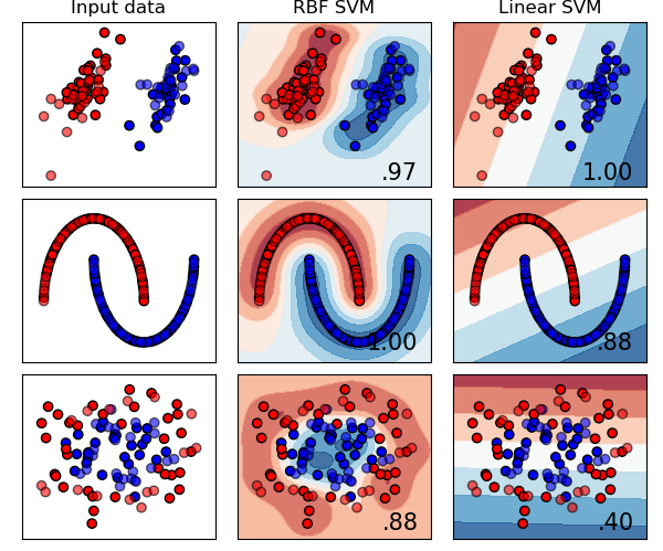
4.1 Simulation With Exact Kernel

The parameters of SVM:

C: 0.6
$\gamma$ of RBF: 2

Here we generate 3 kinds of data. The first row is generated by a Gaussian mixture model. The second row is like a moon generated by Scikit-Learn package. The third one is also generated by Scikit-Learn package and the package generate 2 circles, one is in the inner side and the other one is in the outer side.

The SMO and kernel seem work properly even under noise and nonlinear dataset.

4.2 Simulation With Approximated Kernel

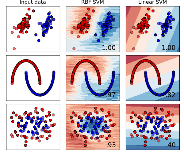
We draw 200 samples from $p(\omega)$ to approximate the RBF kernel. As we can see, the testing accuracies are close to the ones of exact kernels in most of cases.

4.3 Real Dataset

4.3.1 PCA Preprocess

Apply SVM on the “Women’s Clothing E-Commerce Review Dataset” with C = 0.6 and $\gamma$ of RBF kernel = 2, the training accuracy is 82.03% and the testing accuracy is 81.54%. The accuracy, loss and, the movement of variables are showed in the following graph.

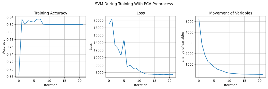
As we can see, the movement of variable gets smaller during training and converge around 50 and the accuracy remains about 82%.

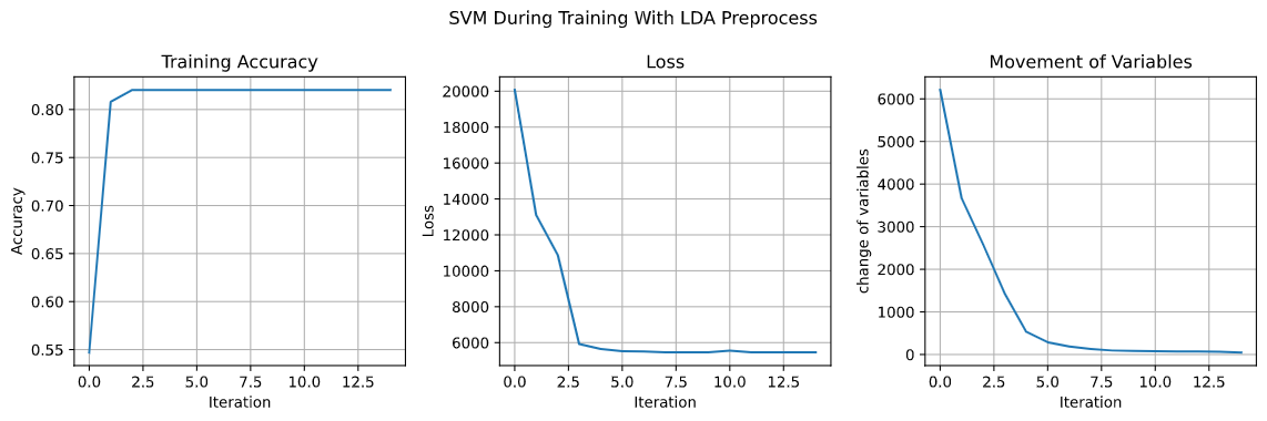
4.3.2 LDA Preprocess

The training accuracy is also 82.03% and the testing accuracy is 81.54%, but the curves are smoother than the ones of PCA.

A Review of SVM and SMO

1. Abstract

2. Sequential Minimal Optimization(SMO)

2.1 Notation

2.2 Step 1. Update 2 Variable

2.3 Step 2. Clip with Bosk Constraint

2.4 Step 3. Update Bias

2.5 Pseudo Code

3. Fourier Kernel Approximation

3.1 Bochner’s Theorem

3.2 Theorem 1

4. Experiments

4.1 Simulation With Exact Kernel

4.2 Simulation With Approximated Kernel

4.3 Real Dataset

COMMENTS

Your comments will encouage me to share more~~

1. Abstract#

2. Sequential Minimal Optimization(SMO)#

2.1 Notation#

2.2 Step 1. Update 2 Variable#

2.3 Step 2. Clip with Bosk Constraint#

2.4 Step 3. Update Bias#

2.5 Pseudo Code#

3. Fourier Kernel Approximation#

3.1 Bochner’s Theorem#

3.2 Theorem 1#

4. Experiments#

4.1 Simulation With Exact Kernel#

4.2 Simulation With Approximated Kernel#

4.3 Real Dataset#

COMMENTS

Your comments will encouage me to share more~~

1. Abstract

2. Sequential Minimal Optimization(SMO)

2.1 Notation

2.2 Step 1. Update 2 Variable

2.3 Step 2. Clip with Bosk Constraint

2.4 Step 3. Update Bias

2.5 Pseudo Code

3. Fourier Kernel Approximation

3.1 Bochner’s Theorem

3.2 Theorem 1

4. Experiments

4.1 Simulation With Exact Kernel

4.2 Simulation With Approximated Kernel

4.3 Real Dataset