Neural Tangent Kernel(NTK)

“In short, NTK represent the changes of the weights before and after the gradient descent update”

Let’s start the journey of revealing the black-box neural networks.

Setup a Neural Network

First of all, we need to define a simple neural network with 2 hidden layers

$$y(x,w)$$

where $y$ is the neural network with weights $w\in {\mathbb{R}}^m$ and, ${x,\overline{y}}_N$ is the dataset which is a set of the input data and the output data with $N$ data points. Since we focus on analyze the weight $w$, we simplify the notation $y(x,w)$ as $y(w)$

Suppose we have a regression task on the network $y(w)$, define

$$L(w)=\frac{1}{N}\frac{1}{2}\Vert y(w)-\overline{y}{\Vert }_2^2$$

where $L(w)$ is our object loss which we want to minimize. Since the term $\frac{1}{N}$ is regardless to our goal, just ignore it and we get a simpler loss function

$$L(w)=\frac{1}{2}\Vert y(w)-\overline{y}{\Vert }_2^2$$

To The Limit of Infinite Width

In order to measure the difference of the weights during training the neural network, we define a normalized metric as following

$$\frac{\Vert w_n-w_0{\Vert }_2}{\Vert w_0{\Vert }_2}$$

where $w_n$ and $w_0$ are the weights at n-th training iteration and the initial weights. $\Vert w_n-w_0{\Vert }_2$ means the quantity of the differnce between parameters $w_n$ and $w_0$ and it is normalized by the 2-norm $\Vert w_0{\Vert }_2$

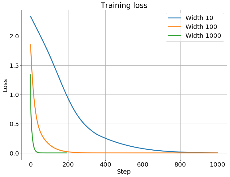
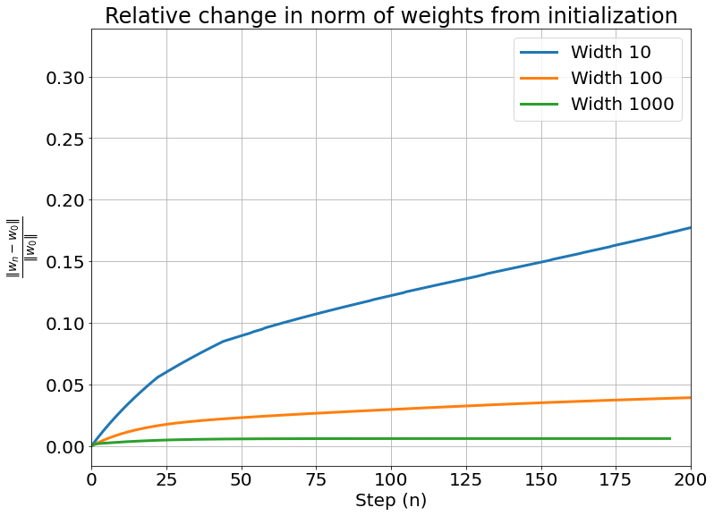
As we can see, the difference of the weights during training decrease as the width of network grows. As a result, the trained weights should be very close to the inital weights $w_0$ as the width of network goes to infinity.

Apply Taylor Expansion

We’ve known the Taylor expansion is

$$f(x)=\sum _{n=0}^{\mathrm{\infty }}\frac{f^n(a)}{n!}(x-a{)}^n$$

A function $f(w)$ expanded on the $w_0$ with first order approximation is

$$f(w)\approx f(w_0)+\frac{df(w_0)}{dw}(w-w_0)$$

It is trivial that if $w$ is a vector, we need to replace the derivative $\frac{df(w_0)}{dw}$ with gradient ${\mathrm{\nabla }}_{w}f(w_0{)}^{\mathrm{\top }}$

$$f(w)\approx f(w_0)+{\mathrm{\nabla }}_{w}f(w_0{)}^{\mathrm{\top }}(w-w_0)$$

Apply to the network $y(w)$

$$y(w)\approx y(w_0)+{\mathrm{\nabla }}_{w}y(w_0{)}^{\mathrm{\top }}(w-w_0)$$

where ${\mathrm{\nabla }}_{w}y(w_0)$ and $y(w_0)$ are constants.

Thus, the Taylor expansion of $y(w)$ is just a linear model. Though the expansion around $w_0$ is regardless to the proof of NTK, it is still a useful tool to analyze the accuracy of the linear approximation with infinite-wide network.

However, the most difficult thing is how can we guarantee the approximation is accurate enough? It is so complex that I wouldn’t put it in this article but I will provide an intuitive explaination of what does NTK mean? in the following article. Please keep reading it if you are interested in it.

An Simpler Explaination Without Flow

Simply, we only consider a 1-dimension network $f(x,w),w,x,\overline{y}\in \mathbb{R}$ for a dataset $x\in X,\overline{y}\in \overline{Y}$ which are input data points and output data points respectively.

First of all, let’s define the loss function of a neural network

$$L_1(x,w)=\frac{1}{2}\Vert f(x,w)-\overline{y}{\Vert }_2^2$$

The gradient descent is

$$w_{t+1}=w_0+\eta \frac{d{L}_1(x,w)}{dw}$$ $$=w_0+\eta (f(x,w)-\overline{y})\frac{df(x,w)}{dw}$$

where $\eta$ is the learning rate.

NTK represent the changes of the weights before and after the gradient descent update. Thus, the changes of weights can be defined as

$$li{m}_{\eta \to 0}\frac{f(x,w+\eta \frac{d{L}_1(x^{\prime },w)}{dw})-f(x,w)}{\eta }$$

$$=li{m}_{\eta \to 0}\frac{f(x,w+\eta (f(x^{\prime },w)-\overline{y})\frac{df(x^{\prime },w)}{dw})-f(x,w)}{\eta }$$

To simplify the notation, let $\eta (f(x^{\prime },w)-\overline{y})\frac{df(x^{\prime },w)}{dw})=\mathrm{\Delta }w$.

We can derive

$$li{m}_{\eta \to 0}\frac{f(x,w+\eta (f(x^{\prime },w)-\overline{y})\frac{df(x^{\prime },w)}{dw})-f(x,w)}{\eta }$$

$$=li{m}_{\eta \to 0}\frac{f(x,w+\mathrm{\Delta }w)-f(x,w)}{\eta }$$

Suppose the learning rate $\eta$ is small enough and thus, $w\approx w+\mathrm{\Delta }w$. We can expand around $w+\mathrm{\Delta }w$ with Taylor expansion

$$f(x,w)\approx f(x,w+\mathrm{\Delta }w)+\frac{df(x,w+\mathrm{\Delta }w)}{dw}(w-(w+\mathrm{\Delta }w))$$

$$=f(x,w+\mathrm{\Delta }w)-\frac{df(x,w+\mathrm{\Delta }w)}{dw}\mathrm{\Delta }w$$

We can get

$$li{m}_{\eta \to 0}\frac{f(x,w+\mathrm{\Delta }w)-f(x,w)}{\eta }$$

$$=li{m}_{\eta \to 0}\frac{f(x,w+\mathrm{\Delta }w)-(f(x,w+\mathrm{\Delta }w)-\frac{df(x,w+\mathrm{\Delta }w)}{dw}\mathrm{\Delta }w)}{\eta }$$

$$=li{m}_{\eta \to 0}\frac{1}{\eta }\frac{df(x,w+\mathrm{\Delta }w)}{dw}\mathrm{\Delta }w$$

$$=li{m}_{\eta \to 0}\frac{df(x,w+\eta (f(x^{\prime },w)-\overline{y})\frac{df(x^{\prime },w)}{dw})}{dw}(f(x^{\prime },w)-\overline{y})\frac{df(x^{\prime },w)}{dw}$$

$$=\frac{df(x,w)}{dw}(f(x^{\prime },w)-\overline{y})\frac{df(x^{\prime },w)}{dw}$$

Since the weight almost not change, let $w=w_0$ and NTK is defined as

$$k_1^{NTK}(x,x^{\prime })=\frac{df(x,w)}{dw}\frac{df(x^{\prime },w)}{dw}=\frac{df(x,w_0)}{dw}\frac{df(x^{\prime },w_0)}{dw}$$

Since $f(x^{\prime },w)-\overline{y}$ would be very close to 0 while MSE is close to 0, we can simply ignore it. It is trivial that NTK represent the changes of weights before and after gradient descent. It measure the difference of weights quantitatively and thus we can approximate the process of gradient descent with Gaussian process.

Flow And Vector Field

So far, we’ve shown the neural tangent kernel on 1-width network. To move forward to the infinite-wide network, we need 2 tools to help us analyzing the process of gradient descent in high-dimensionalal. As a result, before diving into NTK more deeply, we need to understand what is Gradient Flow and Vector Field.

Vector Field

Define a space $\chi \in {\mathbb{R}}^d$ with d dimensions and a point of the space $x\in {\mathbb{R}}^d$. A hyperplane $f(x)f:\chi \to \mathbb{R}$. As we want to find the global minimal point $x^{\ast }$

$$x^{\ast }=\underset{x\in X}{\arg min}f(x)$$

The gradient of the hyperplane ${\mathrm{\nabla }}_{x}f:\chi \to {\mathbb{R}}^d$ represent the gradients of each point on the hyperplane $f$.

Then, we define a vector field $F:\chi \to {\mathbb{R}}^d$ assigning the velocity vector to each points of the space. Mathmatically, the vector field $F$ has the same function space as the gradient ${\mathrm{\nabla }}_{x}f$. As a result, we can also see the gradient ${\mathrm{\nabla }}_{x}f$ as a vector field $-{\mathrm{\nabla }}_{x}f=F(x)$ which assigns the velocity vector $v\in \mathbb{R}$ to each point $x\in \chi$.

$$F(x)=-{\mathrm{\nabla }}_{x}f(x)=v$$

A hyperplane and the gradients can be illustrated as the following figure. The orange surface represents the hyperplane $f$ and the corresponding gradient ${\mathrm{\nabla }}_{x}f$ of each points $x\in \chi$ on the hyperplane $f$ is the blue arrows in the bottom. Note that the gradients ${\mathrm{\nabla }}_{x}f(x)$ here are ascent while gradients of our optimization problem are descent $-{\mathrm{\nabla }}_{x}f(x)$. They have oppsite direction. Intuitively, the gradients represent the direction and steepness of the points on the hyperplane while the vector field is the velocity vector of the points. Mathmatically, the gradients and the vector field have the same function space, so we let them be equal but not due to the physical perspective.

Then we introduce another variable time. Let $c(t)$ for $c:\mathbb{R}\to {\mathbb{R}}^d$ represent the dynamics of along the time $t$. The function $c(t)$ gives the position in the space $\chi \in {\mathbb{R}}^d$ along time $t$.

As a result, we know

$$c(t+\delta )=c(t)+\delta F(c(t))=c(t)-\delta {\mathrm{\nabla }}_{x}f(c(t))$$

where $\delta$ represent the time-step of 2 positions. $\delta F(c(t))=-\delta {\mathrm{\nabla }}_{x}f(c(t))$ means time products velocity vector and then get the movment vector during the time $\delta$.

Gradient Flow

The gradient flow is defined as

$$\dot{X}(t)=F(c(t))=-{\mathrm{\nabla }}_{x}f(c(t))=-{\mathrm{\nabla }}_{x}f(c(t))\dot{c}(t)=-{\mathrm{\nabla }}_{x}f(c(t))\frac{dc(t)}{dt}$$

The gradient flow describe changing gradients along time.

Combined With Gradient Flow

We’ve know the update of the gradient descent is

$$w_{t+1}=w_t-\eta {\mathrm{\nabla }}_{w}L(w_t)$$

Let the function $w(t)=w_t$ and define the gradient flow over weights is $\dot{w}(t)$

$$\dot{w}(t)=-{\mathrm{\nabla }}_{w}L(w(t))$$

Actually, the meaning of the gradient flow $\dot{w}(t)=\frac{dw(t)}{dt}$ is likey the changing direction of gradient descent along time.

We expand the gradient of the loss function with chain rule

$$\dot{w}(t)=-{\mathrm{\nabla }}_{w}L(w(t))$$

$$=-{\mathrm{\nabla }}_w\frac{1}{2}\Vert y(w(t))-\overline{y}{\Vert }_2^2$$

$$=-\frac{1}{2}\cdot 2{\mathrm{\nabla }}_{w}y(w(t))(y(w(t))-\overline{y})$$

$$=-{\mathrm{\nabla }}_{w}y(w(t))(y(w(t))-\overline{y})$$

Now we can derive the flow of the network $\dot{y}(w(t))$

$$\dot{y}(w(t))={\mathrm{\nabla }}_{w}y(w(t){)}^{\mathrm{\top }}\dot{w}(t)$$

$$=-{\mathrm{\nabla }}_{w}y(w(t){)}^{\mathrm{\top }}{\mathrm{\nabla }}_{w}y(w)(y(w(t))-\overline{y})$$

$$=-{\mathrm{\nabla }}_{w}y(w(t){)}^{\mathrm{\top }}{\mathrm{\nabla }}_{w}y(w(t))(y(w(t))-\overline{y})$$

To simplify the notation, we replace the dynamics $w(t)$ with $w_t$.

$$w(t)=w_t$$

Thus, we get

$$\dot{y}(w_t)=-{\mathrm{\nabla }}_{w}y(w_t{)}^{\mathrm{\top }}{\mathrm{\nabla }}_{w}y(w_t)(y(w_t)-\overline{y})$$

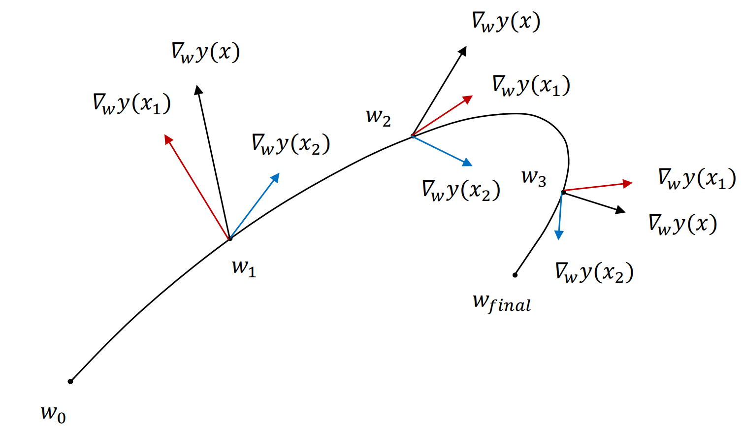
However, we’ve known the mathmatical form of the flow $\dot{y}(w_t)$, but what’s the meaning of the flow $\dot{y}(w_t)$? Well, we can see the updated weights $w_t$ during the gradient descent as a trajectory in a high-dimensional space. Since the learning rate $\eta$ is quite small, the the difference of weights $w_t$ between before and after the gradient descent is very small. As a result, we can see the discrete porgress of the graient descent as a continuous trjectory like the following figure. The flow over the neural network $\dot{y}(w_t)$ is actually the tangent line of $w_t$. The flow $\dot{y}(w_t)$ describe the velocity vector of the point $w_t$ and can predicts close-enough next point $w_{t+1}$.

Since $y(w_t)-\overline{y}$ would be very close to 0, too while MSE is close to 0, we can simply ignore it.

Actually, we are now very close to the neural tangent kernel(NTK). The NTK is a kernel matrix defined as

$${\mathit{K}}_{\mathit{N}\mathit{T}\mathit{K}}\mathbf{(}\mathit{x}\mathbf{,}{\mathit{x}}^{\mathbf{\prime }}\mathbf{)}={\mathrm{\nabla }}_{w}y(x,w_t{)}^{\mathrm{\top }}{\mathrm{\nabla }}_{w}y(x^{\prime },w_t)$$

Since the weights of the infinite-wide network doesn’t change during the training.

$$y(w_t)\approx y(w_0)$$

We get

$$-{\mathrm{\nabla }}_{w}y(w_t{)}^{\mathrm{\top }}{\mathrm{\nabla }}_{w}y(w_t)\approx -{\mathrm{\nabla }}_{w}y(w_0{)}^{\mathrm{\top }}{\mathrm{\nabla }}_{w}y(w_0)=-{\mathrm{\nabla }}_{w}y(x,w_0{)}^{\mathrm{\top }}{\mathrm{\nabla }}_{w}y(x^{\prime },w_0)$$

$$={\mathit{K}}_{\mathit{N}\mathit{T}\mathit{K}}\mathbf{(}\mathit{x}\mathbf{,}{\mathit{x}}^{\mathbf{\prime }}\mathbf{)}$$

Again, ${\mathit{K}}_{\mathit{N}\mathit{T}\mathit{K}}\mathbf{(}\mathit{x}\mathbf{,}{\mathit{x}}^{\mathbf{\prime }}\mathbf{)}$ is the Neural Tangent Kernel, NTK.

The way here to measure the distance between 2 tangents is the Cosine Similarity with inner product. The cosine value of 2 identical vector is 1 and 2 orthorgonal vectors is 0 which are totally different. With an additional minus sign, we can regard the negative similarity as a kind of distance.

To summary, the weights of an infinite-wide network almost don’t change during training. As a result, the kernel always stay almost the same. We can use NTK to analyze many properties of neural network and the neural networks are no longer black boxes.

Papers

NNGP

• Deep Neural Networks as Gaussian Processes

NTK

• Wide Neural Networks of Any Depth Evolve as Linear Models Under Gradient Descent

Reference

Thank for the following posts / people sincerely.

Gaussian Distribution

• StackExchange - Product of two multivariate normal distribution

NNGP

• Deep Gaussian Processes
• Gonzalo Mateo García - Deep Neural Networks as Gaussian Processes
• Deep Gaussian Processes for Machine Learning

NTK

• Understanding the Neural Tangent Kernel By Rajat’s Blog
  • Code for the blog rajatvd/NTK
• Ultra-Wide Deep Nets and the Neural Tangent Kernel (NTK)
• CMU ML Blog: Ultra-Wide Deep Nets and the Neural Tangent Kernel (NTK)
• Some Intuition on the Neural Tangent Kernel
• 直观理解Neural Tangent Kernel

Flow

• Let it flow - Gradient flow and gradient descent

• Max Planck Science - Gradient Flow I

• StackExchange - gradient flow and what is, for example, L2 gradient?

Taylor Expansion

• Taylor series expansion