Note: the code in R is on my Github

3. Variational Bayesian Gaussian Mixture Model(VB-GMM)

3.1 Graphical Model

Gaussian Mixture Model & Clustering

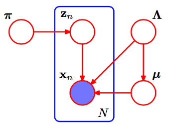
The variational Bayesian Gaussian mixture model(VB-GMM) can be represented as the above graphical model. We see each data point as a Gaussian mixture distribution with $K$ components. We also denote the number of data points as $N$. Each $x_n$ is a Gaussian mixture distribution with a weight $\pi_n$ corresponds to a data point. $z_n$ is an one-hot latent variable that indicates which cluster(component) does the data point belongs to. Finally, A component $k$ follows the Gaussian distribution with mean $\mu_k$ and covariance matrix $\Lambda_k$. $\Lambda = { \Lambda_1, …, \Lambda_K }$ and $\mu = { \mu_1, …, \mu_K }$ are vectors denote the parameters of Gaussian mixture distribution.

Thus, the joint distribution of the VB-GMM is

$$ p(X, Z, \pi, \mu, \Lambda) = p(X | Z, \pi, \mu, \Lambda) p(Z | \pi) p(\pi) p(\mu | \Lambda) p(\Lambda) $$

$p(X | Z, \pi, \mu, \Lambda)$ denotes the Gaussian mixture model given on the latent variables and parameters. $p(Z | \pi)$ denotes the latent variables. As for priors, $p(\pi)$ denotes the prior distribution on the latent variables $Z$ and $p(\mu | \Lambda) p(\Lambda)$ denotes the priors distribution on the Gaussian distribution $X$.

3.2 Gaussian Mixture Model

Suppose each data point $x_n \in \mathbb{R}^D$ has dimension $D$. We define the latent variables $Z = { z_1, …, z_N }, Z \in \mathbb{R}^{N \times K}$, where $z_i ={z_{i1}, …, z_{iK} }, z_i \in \mathbb{R}^K, z_{ij} \in { 0, 1}$. Each $z_{i}$ is a vector containing k binary variables. $z_i$ can be seen as an one-hot encoding that indicates which cluster belongs to. As for $\pi \in \mathbb{R}^K$, $\pi$ is the weight of the Gaussian mixture model of each component.

$$ p(Z | \pi) = \prod_{n=1}^{N}\prod_{k=1}^{K}\pi_{k}^{z_{nk}} $$

Then, we define the components of the Gaussian mixture model. Each component follows Gaussian distribution and is parametrized by the mean $\mu_k$ and covariance matrix $\Lambda_k^{-1}$. Thus, the conditional distribution of the observed data $X \in \mathbb{R}^{N \times D}$, given the variables $Z, \mu, \Lambda$ is

$$ p(X | Z, \mu, \Lambda) = \prod_{n=1}^{N} \prod_{k=1}^{K} \mathcal{N}(x_{n} | \mu_{k}, \Lambda_{k}^{-1})^{z_{nk}} $$

where data $X$ contains $N$ data points and $D$ dimensions, parameter $\mu \in \mathbb{R}^K, \mu = { \mu_1, …, \mu_K }$ and $\Lambda \in \mathbb{R}^{K \times D \times D}, \Lambda_k \in \mathbb{R}^{D \times D}, \Lambda = { \Lambda_1, …, \Lambda_K }$ are the mean and the covariance matrix of each component of Gaussian mixture model.

3.3 Dirichlet Distribution

Next, we introduce another prior over the parameters. We choose the symmetric Dirichlet distribution over the mixing proportions $\pi$. Support $x_1, …, x_K$ where $x_i \in (0, 1)$ and $\sum^K_{i=1} x_i = 1, K > 2$ with parameters $\alpha_1, …, \alpha_K > 0$

$$ X \sim \mathcal{Dir}(\alpha) = \frac{1}{B(\alpha)} \prod^K_{i=1} x^{\alpha_i - 1}_{i} $$

where the Beta function $B(\alpha)=\frac{\prod^K_{i=1} \Gamma(\alpha_i)}{\Gamma(\sum^K_{i=1} \alpha_i)}$ and $\alpha$ and $X$ are a set of random variables that $\alpha = { \alpha_1, …, \alpha_K}$ and $X = { X_1, …, X_K}$. Note that $x_i$ is a sample value generated by $X_i$.

Expectation

The mean of the Dirichlet distribution is

$$ E[X_i] = \frac{\alpha_i}{\sum^K_{k=1} \alpha_k} $$

$$ E[ln \ X_i] = \psi(\alpha_i) - \psi(\sum^K_{k=1} \alpha_k) $$

where $\psi$ is digamma function

$$ \psi(x) = \frac{d}{dx} ln(\Gamma(x)) = \frac{\Gamma’(x)}{\Gamma(x)} \approx ln(x) - \frac{1}{2x} $$

Symmetric Dirichlet distribution

In order to reduce the number of initial parameters, we use Symmetric Dirichlet distribution which is a special form of Dirichlet distribution that defined as the following

$$ X \sim \mathcal{SymmDir}(\alpha_0) = \frac{\Gamma(\alpha_0 K)}{\Gamma(\alpha_0)^K} \prod^K_{i=1} x^{\alpha_0-1}i = f(x_1, …, x{K-1}; \alpha_0) $$ where $X = { X_1, …, X_{K-1} }$. The $\alpha$ parameter of the symmetric Dirichlet is a scalar which means all the elements $\alpha_i$ of the $\alpha$ are the same $\alpha = { \alpha_0, …, \alpha_0 }$.

With Gaussian Mixture Model

Thus, we can model the distribution of the weights of Gaussian mixture model as a symmetric Dirichlet distribution.

$$ p(\pi) = \mathcal{Dir}(\pi | \alpha_0) = \frac{1}{B(\alpha_0)} \prod^K_{k=1} \pi^{\alpha_0 - 1}{k} = C(\alpha_0) \prod^K{k=1} \pi^{\alpha_0 - 1}_{k} $$

3.4 Gaussian-Wishart Distribution

If a normal distribution whose parameters follow the Wishart distribution. It is called Gaussian-Wishart distribution. Support $\mu \in \mathbb{R}^D$ and $\Lambda \in \mathbb{R}^{D \times D}$, they are generated from Gaussian-Wishart distribution which is defined as

$$ (\mu, \Lambda) \sim \mathcal{NW}(m_0, \beta_0, W_0, \nu_0) = \mathcal{N}(\mu | m_0, (\beta_0 \Lambda)^{-1} )\mathcal{W}(\Lambda | W_0, \nu_0) $$

where $m_0 \in \mathbb{R}^D$ is the location, $W \in \mathbb{R}^{D \times D}$ represent the scale matrix, $\beta_0 \in \mathbb{R}, \beta_0 > 0$, and $\nu \in \mathbb{R}, \nu > D - 1$.

Posterior

After making $n$ observations ${ x_1, …, x_n }$ with mean $\bar{x} = \frac{1}{n} \sum_{i=1}^{n} x_i$, the posterior distribution of the parameters is

$$ (\mu, \Lambda) \sim \mathcal{NW}(m_n, \beta_n, W_n, \nu_n) $$

where

$$ \beta_n = \beta_0 + n $$

$$ m_n = \frac{\beta_0 m_0 + n \bar{x}}{\beta_0 + n} $$

$$ \nu_n = \nu_0 + n $$

$$W^{-1}_n = W^{-1}_0 + \sum_{i=1}^{n} (x_i - \bar{x}) (x_i - \bar{x})^{\top} + \frac{n \beta_0}{n + \beta_0} (\bar{x} - m_0) (\bar{x} - m_0)^{\top}$$

With Gaussian Mixture Model

We define the Gaussian mixture model with Gaussian-Wishart prior.

$$ p(\mu, \Lambda) = p(\mu | \Lambda) p(\Lambda) = \prod^K_{k=1} \mathcal{N}(\mu_k | m_0, (\beta_0 \Lambda_k)^{-1}) \mathcal{W}(\Lambda_k | W_0, \nu_0) $$

3.5 The Algorithm

E-Step

E-Step aims to update the variational distribution on latent variables $Z$

$$ ln \ q(Z; \phi^{Z}) \propto \mathbb{E}_{q(\theta; \phi^{\theta})} [log \ p(Y, Z, \theta)] $$

Thus, we can derive

$$ ln\ q(Z) \propto \mathbb{E}_{\pi, \mu, \Lambda} [\text{ln};p(X, Z, \pi, \mu, \Lambda)] $$

$$= \mathbb{E}_{\pi} [ln \ p(Z | \pi)] + \mathbb{E}_{\mu, \Lambda}[ln \ p(X | Z, \mu, \Lambda)] + \mathbb{E}_{\pi, \mu, \Lambda}[ln \ p(\pi, \mu, \Lambda)]$$

$$= \mathbb{E}_{\pi} [ln \ p(Z | \pi)] + \mathbb{E}_{\mu, \Lambda}[ln \ p(X | Z, \mu, \Lambda)] + C$$

where $C$ is a constant,

$$\mathbb{E}_{\pi} [ln \ p(Z | \pi)] = \mathbb{E}_{\pi} \Big[ ln \ \prod_{n=1}^{N}\prod_{k=1}^{K}\pi_{k}^{z_{nk}} \Big]$$

$$= \mathbb{E}_{\pi} \Big[ \sum_{n=1}^{N}\sum_{k=1}^{K} z_{nk} \ ln \ \pi_{k} \Big]$$

$$ = \sum_{n=1}^{N}\sum_{k=1}^{K} z_{nk} \ \mathbb{E}{\pi} [ln \ \pi{k}] $$

and

$$\mathbb{E}_{\mu, \Lambda}[ln \ p(X | Z, \mu, \Lambda)] = \mathbb{E}_{\mu, \Lambda} \Big[ ln \ \prod_{n=1}^{N} \prod_{k=1}^{K} \mathcal{N}(x_{n} | \mu_{k}, \Lambda_{k}^{-1})^{z_{nk}} \Big]$$

$$ = \sum_{n=1}^{N} \sum_{k=1}^{K} z_{nk} \ \mathbb{E}_{\mu_k, \Lambda_k} \Big[ ln \ \frac{e^{-\frac{1}{2} (x_n - \mu_k)^{\top} \Lambda (x_n - \mu_k)}}{\sqrt{(2 \pi)^D det(\Lambda_k^{-1})}} \Big] $$

$$ = \sum_{n=1}^{N} \sum_{k=1}^{K} z_{nk} \ \mathbb{E}_{\mu_k, \Lambda_k} \Big[ -\frac{1}{2} (x_n - \mu_k)^{\top} \Lambda (x_n - \mu_k) - \frac{1}{2} ln ((2 \pi)^D det(\Lambda_k^{-1})) \Big] $$

$$ = \sum_{n=1}^{N} \sum_{k=1}^{K} z_{nk} \Big( -\frac{1}{2}\mathbb{E}{\mu_k, \Lambda_k} \Big[ (x_n - \mu_k)^{\top} \Lambda (x_n - \mu_k) \Big] - \frac{D}{2} ln \ 2 \pi + \mathbb{E}{\Lambda_k} \Big[ ln \ det(\Lambda_k) \Big] \Big) $$

Due to simplification, let

$$ ln \ \rho_{nk} = \mathbb{E}{\pi} [ln \ \pi{k}] - \frac{1}{2}\mathbb{E}{\mu_k, \Lambda_k} \Big[ (x_n - \mu_k)^{\top} \Lambda (x_n - \mu_k) \Big] - \frac{D}{2} ln \ 2 \pi + \mathbb{E}{\Lambda_k} \Big[ ln \ det(\Lambda_k) \Big] $$

Thus,

$$ ln\ q(Z) \propto \sum_{n=1}^{N}\sum_{k=1}^{K} z_{nk} ln \ \rho_{nk} $$

In order to normalize the factor of $\rho_{nk}$, we divide the $\rho_{nk}$ by $\sum_{j=1}^K \rho_{nj}$ and obtain the $r_{nk}$.

$$ ln\ q(Z) \propto \sum_{n=1}^{N}\sum_{k=1}^{K} z_{nk} ln \ r_{nk}, \text{where} \ r_{nk} = \frac{\rho_{nk}}{\sum_{j=1}^K \rho_{nj}} $$

Note that since each data point only belongs to one cluster and $z_{nk}$ is an indicator variable(if data point $i$ belongs to cluster $k$, $z_{ik} = 1$. Otherwise, $z_{ik} = 0$), thus, $\frac{1}{K} \sum_{j=1}^K z_{nj} = \frac{1}{K}$. Therefore, $z_{nk}$ can be seen as a kind of probability that represents how possible does the $n$-th data point belongs to $k$-th cluster. We aims to optimize the expectation $\mathbb{E}[z_{nk}] = 1$, when the $n$-th data point belongs to $k$-th cluster.

$$\mathbb{E}_{z_{nk}} [z_{nk}] = r_{nk}$$

For convenience, we also define some useful variables.

$$ N_k = \sum_{n=1}^N r_{nk}, \quad \bar{x}k = \frac{1}{N_k} \sum{n=1}^N r_{nk} x_n, \quad S_k = \frac{1}{N_k} r_{nk} (x_n - \bar{x}_k) (x_n - \bar{x}_k)^{\top} $$

M-Step

E-Step aims to update the variational distribution on variables $\theta$

$$ ln \ q(\theta; \phi^{\theta}) \propto \mathbb{E}_{q(Z; \phi^{Z})} [log \ p(Y, Z, \theta)] $$

Thus, we can derive

$$ ln\ q(\pi, \mu, \Lambda) \propto \mathbb{E}_{Z} [ln \ p(X, Z, \pi, \mu, \Lambda)] $$

$$= \mathbb{E}_{Z} [ln \ p(X | Z, \pi, \mu, \Lambda)] + \mathbb{E}_{Z} [ln \ p(Z | \pi)] + \mathbb{E}_{Z} [ln \ p(\pi)] + \mathbb{E}_{Z} [ln \ p(\mu, \Lambda)]$$

We assume the joint distribution of parameters follows mean field theorem such that the parameters of each component are independent $q(\pi, \mu, \Lambda) = q(\pi) \prod_{i=1}^N q(\mu_i, \Lambda_i)$. With it, the problem would be easier to solve.

The Posterior of Dirichlet Distribution

$$\mathbb{E}_{Z} [ln \ q(Z | \pi)] + \mathbb{E}_{Z} [ln \ q(\pi)]$$

$$= \mathbb{E}_Z \Big[ ln \ \frac{1}{B(\alpha_0)} \prod^K_{k=1} \pi^{\alpha_0 - 1}_{k} + ln \ \prod_{n=1}^{N}\prod_{k=1}^{K}\pi_{k}^{z_{nk}} \Big]$$

$$= \mathbb{E}_Z \Big[ -ln \ B(\alpha_0) + \sum^K_{k=1} (\alpha_0 - 1) ln \ \pi_{k} + \sum_{n=1}^{N}\sum_{k=1}^{K} z_{nk} ln \ \pi_{k} \Big]$$

$$= -ln \ B(\alpha_0) + \sum^K_{k=1} (\alpha_0 - 1) ln \ \pi_{k} + \sum_{n=1}^{N}\sum_{k=1}^{K} \mathbb{E}_Z [z_{nk}] ln \ \pi_{k}$$

In order to evaluate the posterior distribution with observed data points ${ x_1, …, x_N }$ and the result of E-step, replace the $\mathbb{E}_Z [z_{nk}]$ with $r_{nk}$.

$$ = -ln \ B(\alpha_0) + \sum^K_{k=1} (\alpha_0 - 1) ln \ \pi_{k} + \sum_{k=1}^{K} \sum_{n=1}^{N} r_{nk} ln \ \pi_{k} $$

$$ = -ln \ B(\alpha_0) + \sum^K_{k=1} (\alpha_0 - 1) ln \ \pi_{k} + \sum_{k=1}^{K} \Big( ln \ (\pi_{k}) \sum_{n=1}^{N} r_{nk} \Big) $$

$$ = -ln \ B(\alpha_0) + \sum_{k=1}^{K} (\alpha_0 + N_k - 1) ln \ \pi_{k} $$

Since the posterior distribution of Dirichlet is also Dirichlet, thus we can derive

$$ = ln \ \frac{1}{B(\alpha)} \prod_{k=1}^{K} \pi_{k}^{(\alpha_0 + N_k - 1)} $$

$$ = ln \ \mathcal{Dir}(\pi | \alpha) $$

where $\alpha \in \mathbb{R}^K, \ \alpha = { \alpha_1, …, \alpha_K }, \ \alpha_k = \alpha_0 + N_k$ is the parameter of the Dirichlet distribution.

The Posterior of Gaussian-Wishart Distribution

The posterior distribution parametrized by $m_k, \beta_k, W_k, \nu_k$ is

$$\mathbb{E}_{Z} [ln \ q(\mu, \Lambda)] = \mathbb{E}_{Z}\Big[ ln \ \prod^K_{k=1} \mathcal{N}(\mu_k | m_k, (\beta_k \Lambda_k)^{-1}) \mathcal{W}(\Lambda_k | W_k, \nu_k) \Big]$$

where the parameters of the prior $\lambda$ we’ve given before.

$$ \beta_k = \beta_0 + N_k $$

$$ m_k = \frac{\beta_0 m_0 + N_k \bar{x}_k}{\beta_k} $$

$$ \nu_k = \nu + N_k + 1 $$

$$ W^{-1}_k = W^{-1}_0 + N_k S_k + \frac{N_k \beta_0}{N_k + \beta_0} (\bar{x}_k - m_0) (\bar{x}_k - m_0)^{\top} $$

So far, we’ve derive the parameters of the prior of the bayesian model. Let’s move on to the next iteration of VBEM.

In order to conduct the E-step in the next iteration, we need the parameters of Gaussian mixture model which is denoted by $\theta$. We denote the parameters of Gaussian mixture as $\pi^, \Lambda^$

$$ ln \ \pi_k^* = \mathbb{E}[ln \ \pi_k] = \psi(\alpha_k) - \psi \Big(\sum_{k=1}^K \alpha_k \Big) $$

$$ ln \ \Lambda_k^* = \mathbb{E}[ln \ det(\Lambda_k)] = \sum_{d=1}^{D} \psi \Big( \frac{\nu_{k} + 1 - d}{2} \Big) + D \ ln 2 + ln \ det(W_k) $$

Predict Probability Density

The probability dense function of the VB-GMM is a sum of Student-t distribution. We can derive the PDF from the joint distribution.

$$ q(x^* | X) = \sum_{z^} \int_{\pi} \int_{\mu} \int_{\Lambda} q(x^| z^, \mu, \Lambda) q(z^ | \pi) q(\pi, \mu, \Lambda | X) $$

$$ = \frac{1}{\alpha^} \sum_{k=1}^K \alpha_k \mathcal{St}(x^ | m_k, \frac{(\nu_k + 1 - D) \beta_k}{1 + \beta_k} W_k, \nu_k + 1 - D) $$

VB-GMM Pseudo Code

Repeat until ELBO converge or reach the limit of iteration

E Step

• Compute $ln \ \rho_{nk} = \mathbb{E}{\pi} [ln \ \pi{k}] - \frac{1}{2}\mathbb{E}{\mu_k, \Lambda_k} \Big[ (x_n - \mu_k)^{\top} \Lambda (x_n - \mu_k) \Big] - \frac{D}{2} ln \ 2 \pi + \mathbb{E}{\Lambda_k} \Big[ ln \ det(\Lambda_k) \Big]$ where $1 \leq n \leq N$ and $1 \leq k <K$

• Compute $ln \ r_{nk} = LogSumExp(ln \ \rho_{nk})$

• Compute $r_{nk} = e^{(ln \ \rho_{nk})}$

• Compute $N_k = \sum_{n=1}^N r_{nk}$

• Compute $\bar{x}_k = \frac{1}{N_k} \sum_{n=1}^N r_{nk} x_n$

• Compute $S_k = \frac{1}{N_k} r_{nk} (x_n - \bar{x}_k) (x_n - \bar{x}_k)^{\top}$

M Step

• Update Dirichlet distribution

  • Compute $\alpha_k = \alpha_0 + N_k, \ for \ 1 \leq k \leq K$

• Update Gaussian Mixture distribution

  • Compute $ln \ \pi_k^* = \mathbb{E}[ln \ \pi_k] = \psi(\alpha_k) - \psi \Big(\sum_{k=1}^K \alpha_k \Big)$

• Update Gaussian-Wishart distribution

  • Compute $\beta_k = \beta_0 + N_k, \ for \ 1 \leq k \leq K$

  • Compute $m_k = \frac{\beta_0 m_0 + N_k \bar{x}_k}{\beta_k}, \ for \ 1 \leq k \leq K$

  • Compute $\nu_k = \nu + N_k + 1, \ for \ 1 \leq k \leq K$

  • Compute $W^{-1}_k = W^{-1}_0 + N_k S_k + \frac{N_k \beta_0}{N_k + \beta_0} (\bar{x}_k - m_0) (\bar{x}_k - m_0)^{\top}, \ for \ 1 \leq k \leq K$

• Update posterior for next iteration

  • Compute $ln \ \Lambda_k^* = \sum_{d=1}^{D} \psi \Big( \frac{\nu_{k} + 1 - d}{2} \Big) + D \ ln 2 + ln \ det(W_k), \ for \ 1 \leq k \leq K$

  • Compute $ln \ \pi_k^* = \psi(\alpha_k) - \psi \Big(\sum_{k=1}^K \alpha_k \Big), \ for \ 1 \leq k \leq K$

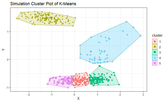
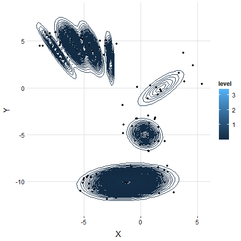
4. Simulation

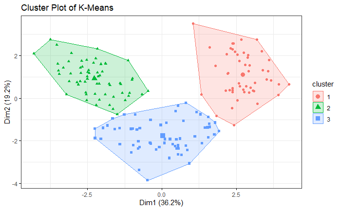
We generate the simulation data by bivariate Gaussian mixture distribution with 5 modals. We use K-means which is given 5 clusters as hyperparameter. VB-GMM out-performs than K-means while clustering an unbalanced dataset. Even though the K-mean already has correct hyperparameters.

VB-GMM not only deals with unbalanced dataset well but also self-adapts to the best number of clusters which is very close to the ground truth.

K-means

VB-GMM

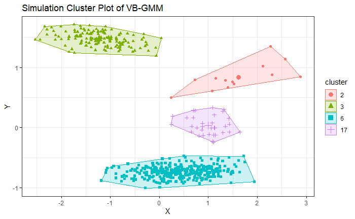
With the animation, we can see the number of clusters of VB-GMM keep reducing until it find a best fit to the dataset. Please refer to the link.

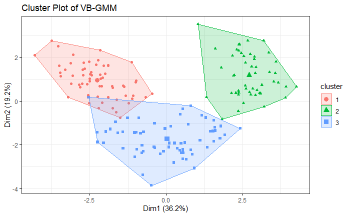
5. Examine on Real Dataset

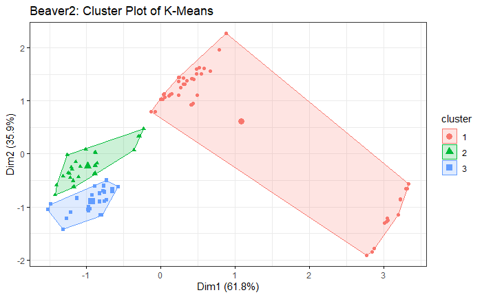
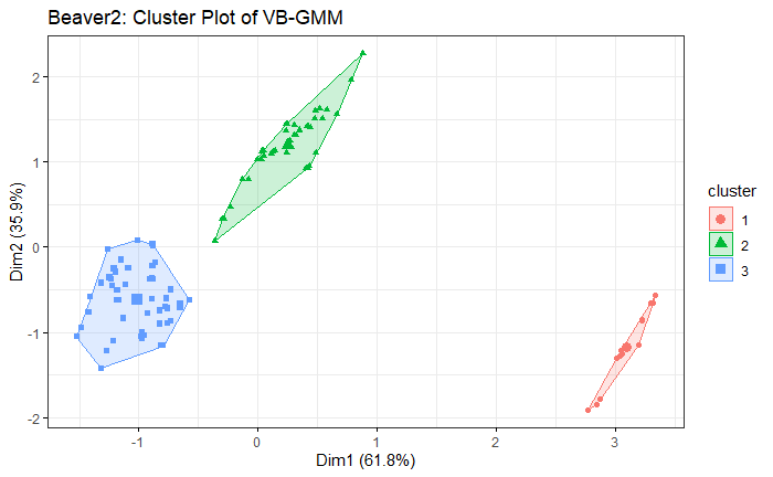
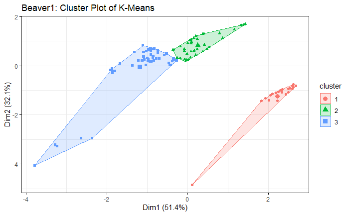
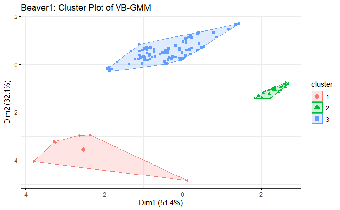
The result is similar to the simulation. VB-GMM usually out-perform than K-means while clustering unbalanced dataset.

Wine Dataset

Beaver1 Dataset

Beaver2 Dataset